Introduction
Once we have our expression matrix, it should be examined to remove poor quality cells which were not detected in the initial processing of the raw reads. Failure to remove low quality cells at this stage may add technical noise which has the potential to obscure the biological signals of interest in the downstream analysis.
Since there is currently no standard method for performing scRNAseq, the expected values for the various QC measures that will be presented here can vary substantially from experiment to experiment. Thus, to perform QC we will be looking for cells which are outliers with respect to the rest of the dataset rather than comparing to independent quality standards. Consequently, care should be taken when comparing quality metrics across datasets collected using different protocols.
Dataset
We'll continue working with the Tabula Muris brain data that we prepared earlier:
import scanpy as sc # import scanpy to handle our AnnData
import pandas as pd # import pandas to handle dataframes
import matplotlib.pyplot as plt # import matplotlib to visualize our qc metrics

# magic incantation to help matplotlib work with our jupyter notebook
%matplotlib inline
adata = sc.read('../data/brain_raw.h5ad')
As an aside, you'll notice that both here and in the previous notebook we read data into python objects using some variation on package.read*, where * indicates that there is some possible suffix. Developers of python data packages that we'll be using today, and many others in the ecosystem try very hard to group objects so that they are discoverable.
One method of discovering functionality in python is to read documentation. Another is to use tab-completion to find similar functions. For reading files, it's usually possible to see what possibilities there are by tab completing package.read, package.load, or package.open. It's unusual for these functions to start with other words.
For writing files, usually the pattern is object.save or object.write. In this case, try using the package.read pattern by tab completing sc.read and see what happens. What about tab completion with the object.write pattern using the adata object we just loaded?
Knowing this pattern is very helpful. Unfortunately, data files containing expression information will often come in all shapes and sizes. Thankfully, developers of these packages are aware of the common types, and may have already designed readers and writers to make them easy to work with. With this knowledge in hand, you'll be well equipped to execute the following tasks on data stored in a broader variety of file formats.
Computing quality control metrics
We'll compute quality metrics and then filter cells and genes accordingly.
The calculate_qc_metrics function returns two dataframes: one containing quality control metrics about cells, and one containing metrics about genes. This function is housed in the 'preprocessing' portion of the SCANPY library, which you can read more about here.
qc = sc.pp.calculate_qc_metrics(adata, qc_vars = ['ERCC'])# this returns a tuple of (cell_qc_dataframe, gene_qc_dataframe)
                                 # ask for the percentage of reads from spike ins

cell_qc_dataframe = qc[0]
gene_qc_dataframe = qc[1]

print('This is the cell quality control dataframe:')
print(cell_qc_dataframe.head(2))

print('\n\n\n\nThis is the gene quality control dataframe:')
print(gene_qc_dataframe.head(2))
plt.hist(cell_qc_dataframe['total_counts'], bins=1000)
plt.xlabel('Total counts')
plt.ylabel('N cells')
plt.axvline(50000, color='red')
# plt.xlim(0,1e6) # Try plotting with and without scaling the x-axis. When is this helpful?
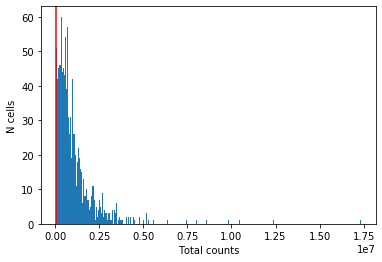
Looks like the authors have already removed cells with fewer than 50,000 reads.
plt.hist(cell_qc_dataframe['n_genes_by_counts'], bins=100)
plt.xlabel('N genes')
plt.ylabel('N cells')
plt.axvline(1000, color='red')

From the plot we conclude that most cells have between ~1,000-5,000 detected genes, which is typical for smartseq2 data. However, this varies by experimental protocol and sequencing depth.
The most notable feature in the above plot is the little peak on the left hand side of the distribution. If detection rates were equal across the cells then the distribution should be approximately normal. Thus, we will remove those cells in the tail of the distribution (fewer than ~1000 detected genes).
Spike-ins
Another measure of cell quality is the ratio between ERCC spike-in RNAs and endogenous RNAs. This ratio can be used to estimate the total amount of RNA in the captured cells. Cells with a high level of spike-in RNAs had low starting amounts of RNA, likely due to the cell being dead or stressed which may result in the RNA being degraded.
Exercise
Plot the distribution of pct_counts_ERCC in this dataset. What do you think is a reasonable threshold?
Solution
plt.hist(cell_qc_dataframe['pct_counts_ERCC'], bins=1000)
plt.xlabel('Percent counts ERCC')
plt.ylabel('N cells')
plt.axvline(10, color='red')
Placing a threshold is always a judgement call. Here, the majority of cells have less than 10% ERCC counts, but there's a long tail of cells that have very high spike-in counts; these are likely dead cells and should be removed.
plt.hist(...)
plt.xlabel(...)
plt.ylabel(...)
plt.axvline(...)
There isn't an automatic function for removing cells with a high percentage of ERCC reads, but we can use a mask to remove them like so:
low_ERCC_mask = (cell_qc_dataframe['pct_counts_ERCC'] < 10)
adata = adata[low_ERCC_mask]
Exercise
Use the SCANPY function sc.pp.filter_cells() to filter cells with fewer 750 genes detected. How many cells does this remove?
_Hint: start with the Parameters list in help(sc.pp.filter_cells)
Solution
print('Started with: \n', adata)
sc.pp.filter_cells(adata, min_genes = 750)
print('Finished with: \n', adata)
help(sc.pp.filter_cells)
Quality control for genes
It is typically a good idea to remove genes whose expression level is considered "undetectable". We define a gene as detectable if at least two cells contain more than 5 reads from the gene. However, the threshold strongly depends on the sequencing depth. It is important to keep in mind that genes must be filtered after cell filtering since some genes may only be detected in poor quality cells.
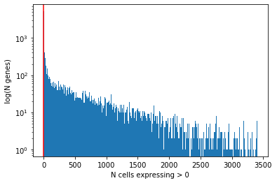
plt.hist(gene_qc_dataframe['n_cells_by_counts'], bins=1000)
plt.xlabel('N cells expressing > 0')
plt.ylabel('log(N genes)') # for visual clarity
plt.axvline(2, color='red')
plt.yscale('log')
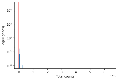
plt.hist(gene_qc_dataframe['total_counts'], bins=1000)
plt.xlabel('Total counts')
plt.ylabel('log(N genes)') # for visual clarity
plt.yscale('log')
plt.axvline(10, color='red')
Exercise
Use the SCANPY function sc.pp.filter_genes() to filter genes according to the criteria above. How many genes does this remove?
_Hint: start with the Parameters list in help(sc.pp.filter_genes)
Solution
print('Started with: \n', adata)
sc.pp.filter_genes(adata, min_cells = 2)
sc.pp.filter_genes(adata, min_counts = 10)
print('Finished with: \n', adata)
help(sc.pp.filter_genes)
# print(adata) ## Final dimensions of the QC'd dataset
adata.write('../data/brain_qc.h5ad')