Normalizing full-length gene sequencing data • cellxgene.census

This tutorial shows you how to fetch full-length gene sequencing data from the Census and normalize it to account for gene length.

Contents

Opening the census
Fetching example full-length sequencing data (Smart-Seq2)
Normalizing expression to account for gene length
Validation through clustering exploration

Opening the census

First we open the Census:

library("Seurat")
census <- cellxgene.census::open_soma()

You can learn more about all of the cellxgene.census methods by accessing their corresponding documentation, for example ?cellxgene.census::open_soma.

Fetching full-length example sequencing data (Smart-Seq)

Let’s get some example data, in this case we’ll fetch all cells from a relatively small dataset derived from the Smart-Seq2 technology which performs full-length gene sequencing:

Collection: Tabula Muris Senis
Dataset: Liver - A single-cell transcriptomic atlas characterizes ageing tissues in the mouse - Smart-seq2

Let’s first find this dataset’s id by using the dataset table of the Census.

liver_dataset <- as.data.frame(
  census$get("census_info")$get("datasets")
  $read(value_filter = "dataset_title == 'Liver - A single-cell transcriptomic atlas characterizes ageing tissues in the mouse - Smart-seq2'")
  $concat()
)
liver_dataset
#>   soma_joinid                        collection_id    collection_name
#> 1         583 0b9d8a04-bb9d-44da-aa27-705bb65b54eb Tabula Muris Senis
#>              collection_doi                           dataset_id
#> 1 10.1038/s41586-020-2496-1 4546e757-34d0-4d17-be06-538318925fcd
#>                     dataset_version_id
#> 1 0a851e26-a629-4e59-9b52-9b4d1ce4440b
#>                                                                                       dataset_title
#> 1 Liver - A single-cell transcriptomic atlas characterizes ageing tissues in the mouse - Smart-seq2
#>                           dataset_h5ad_path dataset_total_cell_count
#> 1 4546e757-34d0-4d17-be06-538318925fcd.h5ad                     2859

Now we can use this id to fetch the data.

liver_dataset_id <- liver_dataset[1, "dataset_id"]
liver_seurat <- cellxgene.census::get_seurat(
  census,
  organism = "Mus musculus",
  obs_value_filter = paste0("dataset_id == '", liver_dataset_id, "'")
)

Let’s make sure this data only contains Smart-Seq2 cells.

table(liver_seurat$assay)
#> 
#> Smart-seq2 
#>       2859

Great! As you can see this a small dataset only containing 2,859 cells. Now let’s proceed to normalize by gene lengths.

Normalizing expression to account for gene length

By default cellxgene_census::get_seurat() fetches all genes in the Census. So let’s first identify the genes that were measured in this dataset and subset the Seurat obect to only include those.

To this goal we can use the “Dataset Presence Matrix” in census$get("census_data")$get("mus_musculus")$ms$get("RNA")$get("feature_dataset_presence_matrix"). This is a boolean matrix N x M where N is the number of datasets, M is the number of genes in the Census, and a 1 entry indicates that a gene was measured in a dataset. (Note that Seurat objects have the transposed layout M x N.)

liver_seurat
#> An object of class Seurat 
#> 52417 features across 2859 samples within 1 assay 
#> Active assay: RNA (52417 features, 0 variable features)
#>  2 layers present: counts, data

Let’s get the genes measured in this dataset.

liver_dataset_joinid <- liver_dataset$soma_joinid[1]
presence_matrix <- cellxgene.census::get_presence_matrix(census, "Mus musculus", "RNA")
presence_matrix <- presence_matrix$take(liver_dataset_joinid)
gene_presence <- as.vector(presence_matrix$get_one_based_matrix())

liver_seurat <- liver_seurat[gene_presence, ]
liver_seurat
#> An object of class Seurat 
#> 17992 features across 2859 samples within 1 assay 
#> Active assay: RNA (17992 features, 0 variable features)
#>  2 layers present: counts, data

We can see that out of all genes in the Census 17,992 were measured in this dataset.

Now let’s normalize these genes by gene length. We can easily do this because the Census has gene lengths included in the gene metadata under feature_length.

GetAssayData(liver_seurat[1:5, 1:5], slot = "data")
#> Warning: The `slot` argument of `GetAssayData()` is deprecated as of SeuratObject 5.0.0.
#> i Please use the `layer` argument instead.
#> This warning is displayed once every 8 hours.
#> Call `lifecycle::last_lifecycle_warnings()` to see where this warning was generated.
#> 5 x 5 sparse Matrix of class "dgCMatrix"
#>                    cell3959639 cell3959640 cell3959641 cell3959642 cell3959643
#> ENSMUSG00000025900           .           .           .           .           .
#> ENSMUSG00000025902           .           .           .           .        2250
#> ENSMUSG00000033845           .         559        1969           .           .
#> ENSMUSG00000025903           .           .           .           .           .
#> ENSMUSG00000033813           .           .         828           1          54

gene_lengths <- liver_seurat$RNA@meta.features$feature_length
liver_seurat <- SetAssayData(
  liver_seurat,
  new.data = sweep(GetAssayData(liver_seurat, slot = "data"), 1, gene_lengths, "/")
)

GetAssayData(liver_seurat[1:5, 1:5], slot = "data")
#> 5 x 5 sparse Matrix of class "dgCMatrix"
#>                    cell3959639 cell3959640 cell3959641  cell3959642 cell3959643
#> ENSMUSG00000025900           .  .            .         .             .         
#> ENSMUSG00000025902           .  .            .         .             0.47150042
#> ENSMUSG00000033845           .  0.06586544   0.2320019 .             .         
#> ENSMUSG00000025903           .  .            .         .             .         
#> ENSMUSG00000033813           .  .            0.2744448 0.0003314551  0.01789857

All done! You can now see that we have real numbers instead of integers.

Validation through clustering exploration

Let’s perform some basic clustering analysis to see if cell types cluster as expected using the normalized counts.

First we do some basic filtering of cells and genes.

cells_per_gene <- rowSums(GetAssayData(liver_seurat, slot = "counts") > 0)
genes_per_cell <- Matrix::colSums(liver_seurat$RNA@counts > 0)
liver_seurat <- liver_seurat[cells_per_gene >= 5, genes_per_cell >= 500]

Then we normalize to account for sequencing depth and transform data to log scale.

liver_seurat <- Seurat::NormalizeData(
  liver_seurat,
  normalization.method = "LogNormalize",
  scale.factor = 10000
)

Then we subset to highly variable genes.

liver_seurat <- Seurat::FindVariableFeatures(
  liver_seurat,
  selection.method = "vst",
  nfeatures = 1000
)

And finally we scale values across the gene axis.

all.genes <- rownames(liver_seurat)
liver_seurat <- Seurat::ScaleData(liver_seurat, features = all.genes)

Now we can proceed to do clustering analysis.

liver_seurat <- RunPCA(
  liver_seurat,
  features = VariableFeatures(object = liver_seurat)
)
liver_seurat <- FindNeighbors(liver_seurat, dims = 1:40)
liver_seurat <- RunUMAP(liver_seurat, dims = 1:40)
DimPlot(liver_seurat, reduction = "umap", group.by = "cell_type")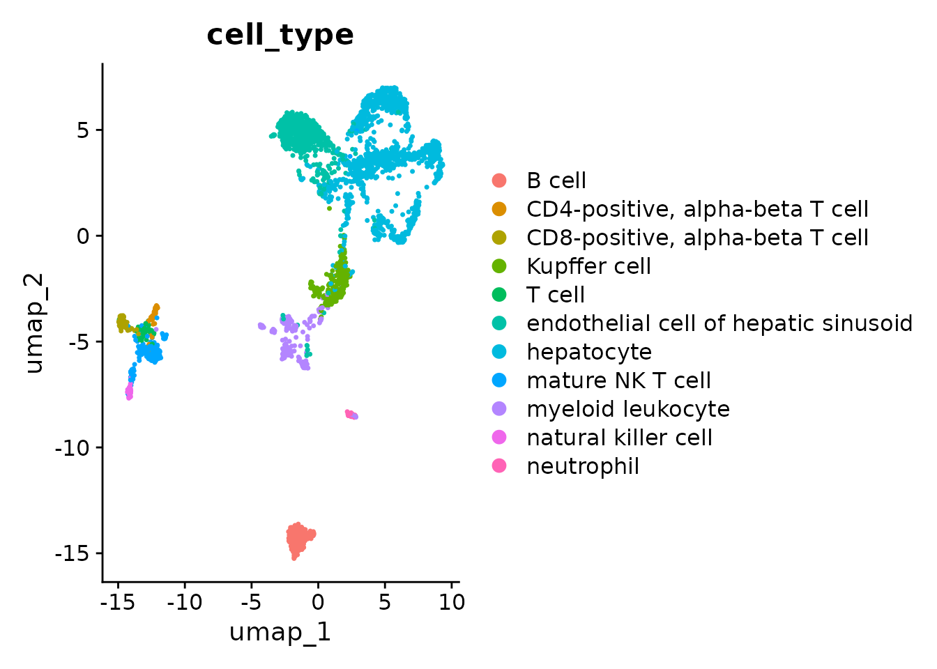

With a few exceptions we can see that all cells from the same cell type cluster near each other which serves as a sanity check for the gene-length normalization that we applied.

Don’t forget to close the census.

census$close()