Find the most similar Census cells in any other data with embeddings vector search

This tutorial demonstrates the experimental API in the Python cellxgene_census package to search Census embeddings using TileDB-Vector-Search indexes. We will generate scVI embeddings for some test cells, search the Census scVI embeddings for nearest neighbors, and use them to predict cell type and tissue of the test cells.

To reproduce this notebook, pip install 'cellxgene_census[experimental]' scvi-tools and obtain the pbmc3k blood cells data and scVI model:

Contents

1. Downloading data and Census scVI model.

2. Loading and embedding pbmc3k cells.

3. Search for similar Census cells.

4. Predicting cell metadata.

⚠️ Note that the Census RNA data includes duplicate cells present across multiple datasets. Duplicate cells can be filtered in or out using the cell metadata variable is_primary_data which is described in the Census schema.

Downloading data and Census scVI model

Download the data first. This the 10X PBMC 3K dataset.

import warnings

warnings.filterwarnings("ignore")

import anndata
import cellxgene_census
import cellxgene_census.experimental
import pandas as pd
import scanpy as sc
import scvi

CENSUS_VERSION = "2024-07-01"

Download the test data which will be used to look for their Census most similar cells. This is the test 10X PMBC dataset.

!mkdir -p data
!wget --no-check-certificate -q -O data/pbmc3k_filtered_gene_bc_matrices.tar.gz http://cf.10xgenomics.com/samples/cell-exp/1.1.0/pbmc3k/pbmc3k_filtered_gene_bc_matrices.tar.gz
!tar -xzf data/pbmc3k_filtered_gene_bc_matrices.tar.gz -C data/

Now download the model corresponding to the census version used in the notebook.

First find S3 location of the model.

with cellxgene_census.open_soma(census_version=CENSUS_VERSION) as census:
    census = cellxgene_census.open_soma(census_version=CENSUS_VERSION)

    scvi_info = cellxgene_census.experimental.get_embedding_metadata_by_name(
        embedding_name="scvi",
        organism="homo_sapiens",
        census_version=CENSUS_VERSION,
    )

scvi_info["model_link"]

's3://cellxgene-contrib-public/models/scvi/2024-07-01/homo_sapiens/model.pt'

Now use that path to download via HTTPs, make sure to update the URL if you change the Census version.

!mkdir -p scvi-human-2024-07-01
!wget --no-check-certificate -q -O scvi-human-2024-07-01/model.pt https://cellxgene-contrib-public.s3.us-west-2.amazonaws.com/models/scvi/2024-07-01/homo_sapiens/model.pt

Loading and embedding pbmc3k cells

Load the pmbc3k cell data into an AnnData:

adata = sc.read_10x_mtx("data/filtered_gene_bc_matrices/hg19/", var_names="gene_ids")
adata.var["ensembl_id"] = adata.var.index
adata.obs["n_counts"] = adata.X.sum(axis=1)
adata.obs["joinid"] = list(range(adata.n_obs))
adata.obs["batch"] = "unassigned"

Run them through the scVI forward pass and extract their latent representation (embedding):

scvi.model.SCVI.prepare_query_anndata(adata, "scvi-human-2024-07-01")
vae_q = scvi.model.SCVI.load_query_data(
    adata,
    "scvi-human-2024-07-01",
)

# This allows for a simple forward pass
vae_q.is_trained = True
latent = vae_q.get_latent_representation()
adata.obsm["scvi"] = latent

INFO     File scvi-human-2024-07-01/model.pt already downloaded
INFO     Found 54.675% reference vars in query data.
INFO     File scvi-human-2024-07-01/model.pt already downloaded

An NVIDIA GPU may be present on this machine, but a CUDA-enabled jaxlib is not installed. Falling back to cpu.

The scVI embedding vectors for each cell are now stored in the scvi obsm layer. Lastly, clean up the AnnData a little:

# filter out missing features
adata = adata[:, adata.var["gene_symbols"].notnull().values].copy()
adata.var.set_index("gene_symbols", inplace=True)
# assign placeholder cell_type and tissue_general labels
adata.var_names = adata.var["ensembl_id"]
adata.obs["cell_type"] = "Query - PBMC 10X"
adata.obs["tissue_general"] = "Query - PBMC 10X"

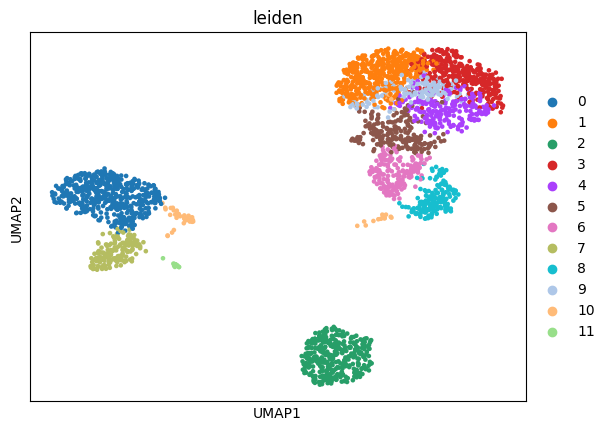
And for visualization, compute leiden clusters on the scVI embeddings. These will come at handy later on.

sc.pp.neighbors(adata, n_neighbors=15, use_rep="scvi")
sc.tl.umap(adata)
sc.tl.leiden(adata)
sc.pl.umap(adata, color="leiden")

Search for similar Census cells

Use the CELLxGENE Census experimental API to search the vector index of scVI embeddings.

%%time
neighbors = cellxgene_census.experimental.find_nearest_obs(
    "scvi", "homo_sapiens", CENSUS_VERSION, query=adata, k=30, memory_GiB=8, nprobe=20
)

CPU times: user 1min 18s, sys: 1min 3s, total: 2min 22s
Wall time: 44.1 s

This accessed the cell embeddings in the scvi obsm layer and searched the latent space for the k nearest neighbors (by Euclidean distance) among the Census cell embeddings, returning the distances and obs soma_joinids (k for each query cell).

neighbors

NeighborObs(distances=array([[0.15405715, 0.16895768, 0.23857602, ..., 0.3158804 , 0.3161367 ,
        0.31640536],
       [0.29017174, 0.3242963 , 0.34604427, ..., 0.56234425, 0.56352013,
        0.56709266],
       [0.40463728, 0.41439083, 0.4177297 , ..., 0.55779415, 0.56181365,
        0.5627153 ],
       ...,
       [0.19712524, 0.2522816 , 0.2780036 , ..., 0.34790507, 0.34811306,
        0.35188618],
       [0.36992368, 0.3832991 , 0.39696082, ..., 0.560152  , 0.564542  ,
        0.5646585 ],
       [0.33078673, 0.3308513 , 0.35727894, ..., 0.52874607, 0.5310725 ,
        0.53260434]], dtype=float32), neighbor_ids=array([[53938900, 56894874, 53904832, ..., 35431931, 34956866, 53863941],
       [ 6276632, 18807209,  7251536, ..., 12705987, 11951694, 11980870],
       [16903285, 21674180, 50898826, ..., 35424173, 44145922, 36066801],
       ...,
       [36336282, 52999747, 53523979, ..., 54143971, 53062159, 46403244],
       [36217923, 46782331, 35719817, ..., 54091908, 46313955, 46545266],
       [35205445, 56547047, 36327798, ..., 34826668, 35829524, 54033347]],
      dtype=uint64))

To explore these results, fetch an AnnData with each query cell’s (single) nearest neighbor in scVI’s latent space, including their embedding vectors:

with cellxgene_census.open_soma(census_version=CENSUS_VERSION) as census:
    neighbors_adata = cellxgene_census.get_anndata(
        census,
        "homo_sapiens",
        "RNA",
        obs_coords=sorted(neighbors.neighbor_ids[:, 0].tolist()),
        obs_embeddings=["scvi"],
        X_name="normalized",
        column_names={"obs": ["soma_joinid", "tissue", "tissue_general", "cell_type"]},
    )
neighbors_adata.var_names = neighbors_adata.var["feature_id"]

Make a UMAP visualization of these nearest neighbors:

sc.pp.neighbors(neighbors_adata, n_neighbors=15, use_rep="scvi")
sc.tl.umap(neighbors_adata)
sc.pl.umap(neighbors_adata, color="tissue_general")

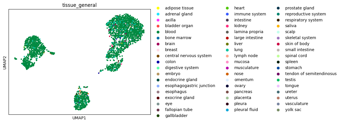
As expected, the nearest neighbors are largely Census blood cells, with some distinct cell type clusters.

Now display the pbmc3k query cells together with their Census nearest neighbors:

adata_concat = anndata.concat([adata, neighbors_adata])
sc.pp.neighbors(adata_concat, n_neighbors=15, use_rep="scvi")
sc.tl.umap(adata_concat)
sc.pl.umap(adata_concat, color=["tissue_general"])

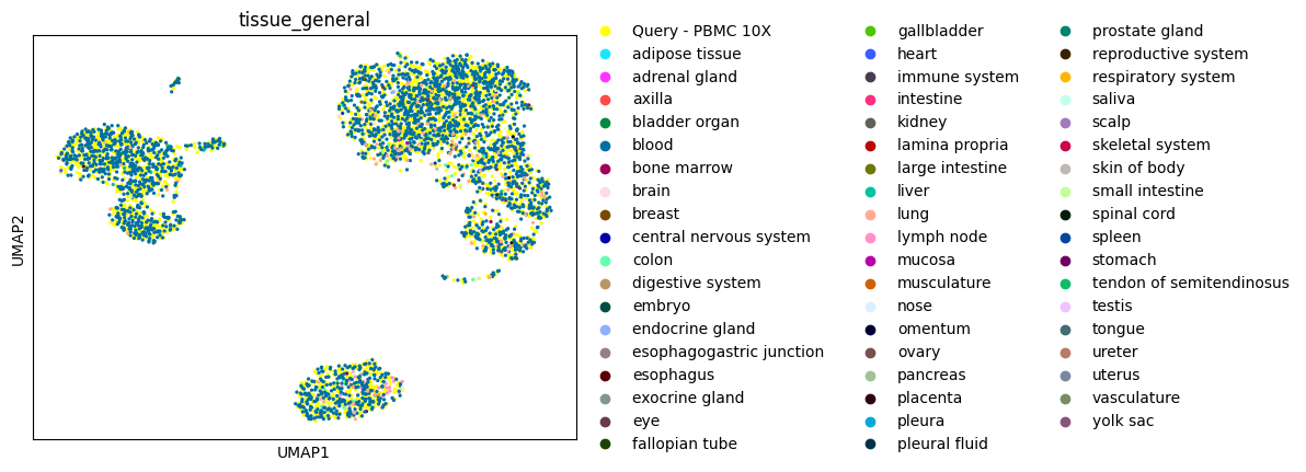
The neighbor clusters appear to correspond to cell type heterogeneity also present in the query.

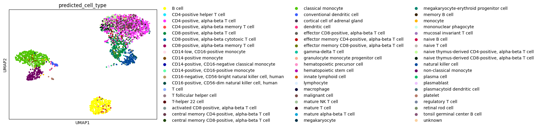
Predicting cell metadata

The experimental API also has a method to predict metadata attributes of the query cells, like tissue_general and cell_type, based on the Census nearest neighbors.

predictions = cellxgene_census.experimental.predict_obs_metadata(
    "homo_sapiens", CENSUS_VERSION, neighbors, ["tissue_general", "cell_type"]
)
predictions

	tissue_general	tissue_general_confidence	cell_type	cell_type_confidence
0	blood	0.866667	CD4-positive, alpha-beta T cell	0.366667
1	lymph node	0.366667	B cell	0.433333
2	blood	0.966667	central memory CD4-positive, alpha-beta T cell	0.266667
3	blood	0.900000	classical monocyte	0.733333
4	blood	0.900000	natural killer cell	0.633333
...	...	...	...	...
2695	blood	0.800000	classical monocyte	0.600000
2696	immune system	0.366667	plasmablast	0.566667
2697	blood	0.966667	B cell	0.633333
2698	blood	0.866667	B cell	0.600000
2699	blood	0.866667	CD4-positive, alpha-beta T cell	0.333333

2700 rows × 4 columns

Unlike the above visualizations of single nearest neighbors, these predictions are informed by each query cell’s k=30 neighbors, with an attached confidence score.

These predictions can be added to the original AnnData object for visualization.

predictions.index = adata.obs.index
predictions = predictions.rename(columns={"cell_type": "predicted_cell_type"})
adata.obs = pd.concat([adata.obs, predictions], axis=1)

sc.pl.umap(adata, color="predicted_cell_type")

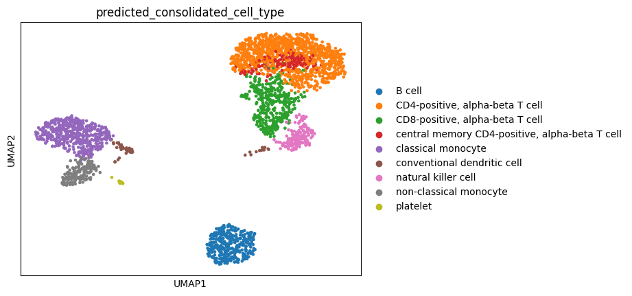
Now the leiden clusters calculated at the beginning can be annotated by popular vote, whereby each cluster gets assigned the most common predicted cell type from the previous step.

adata.obs["predicted_consolidated_cell_type"] = ""
for leiden_cluster in adata.obs["leiden"].drop_duplicates():
    most_popular_type = (
        adata.obs.loc[adata.obs["leiden"] == leiden_cluster,].value_counts("predicted_cell_type").index[0]
    )
    adata.obs.loc[adata.obs["leiden"] == leiden_cluster, "predicted_consolidated_cell_type"] = most_popular_type

sc.pl.umap(adata, color="predicted_consolidated_cell_type")