Accessing Spatial Data in Census

Introduction: Accessing Spatial Data via CELLxGENE Census API

We are excited to announce that spatial data is now accessible in Census. Users can query and retrieve spatial datasets from the CELLxGENE spatial corpus. Currently, the following spatial assays are supported:

Visium
Slide-seq V2

This functionality is available starting from:

CELLxGENE Census: Version v1.16.2
TileDB-SOMA: Version v1.15.5

Key Features

Query Spatial Data: Use the Census spatial object to perform queries and retrieve spatial slides from the CELLxGENE spatial corpus. Filter based on categorical metadata and gene expression.
Export to SpatialData: Retrieved spatial data can be exported to the SpatialData library for further analysis and visualization.

We will now demonstrate how to query the spatial census object, export to SpatialData plot spatial data retrieved from Census.

Environment and dependencies

We recommend that you set up a new environment to avoid conflicts with any existing packages you may have in your regular or system python environment. Here is an example using conda:

conda create --name spatial-census-dev python=3.11 -y # create virtual env
conda activate spatial-census-dev
conda install -c conda-forge jupyterlab # or "pip install jupyterlab" if not using conda

Install

To get started, ensure you have the necessary dependencies installed (we recommend doing this in a virtual environment). You’ll need TileDB-SOMA (v1.15.3 or later) and SpatialData (including the extras for spatial support). You can install them using the following commands:

pip install cellxgene-census "tiledbsoma>=1.15.5" "spatialdata[extra]>=0.2.5"

Load

[1]:

import cellxgene_census
import tiledbsoma
import spatialdata as sd
import spatialdata_plot

import warnings
warnings.filterwarnings("ignore")

/home/ubuntu/miniforge3/envs/census-spatial/lib/python3.11/site-packages/dask/dataframe/__init__.py:31: FutureWarning: The legacy Dask DataFrame implementation is deprecated and will be removed in a future version. Set the configuration option `dataframe.query-planning` to `True` or None to enable the new Dask Dataframe implementation and silence this warning.
  warnings.warn(

[2]:

#versions of required libraries for this tutorial
print("cellxgene_census",cellxgene_census.__version__)
print("tiledbsoma", tiledbsoma.__version__)
print("spatialdata", sd.__version__)
print("spatialdata plot", spatialdata_plot.__version__)

cellxgene_census 1.16.2
tiledbsoma 1.15.5
spatialdata 0.3.0
spatialdata plot 0.2.9

Census Metadata

We can find Census level metadata in the census_info slot. In this slot we can also view a complete list of datasets in this release of the census - note the inclusion of spatial datasets in the sample data table printed below. Additionally, we can print out the keys associated with the census_spatial_sequencing slot giving us access to Visium and Slide seq V2 assays performed in either mouse or human. Also note that for spatial data within census, we make no normalized expression data layer available.

[3]:

with cellxgene_census.open_soma(census_version="2025-01-30") as census:
    #Print Census level metadata
    print("Census level metadata\n")
    print(list(census["census_info"].keys()))

    print("\n")

    print("Census datasets info\n")
    print(census["census_info"]["datasets"].read().concat().to_pandas().head())

    print("\n")

    print("Census spatial keys\n")
    print(list(census["census_spatial_sequencing"].keys()))

    #[optional] not run - spatial data obs metadata table
    #print(census["census_spatial_sequencing"]["homo_sapiens"]["obs"].read().concat().to_pandas().head())

    #[optional] not run - spatial data var metadata table
    #print(census["census_spatial_sequencing"]["homo_sapiens"]["ms"]["RNA"]["var"].read().concat().to_pandas().head())

Census level metadata

['datasets', 'organisms', 'summary', 'summary_cell_counts']


Census datasets info

   soma_joinid                                           citation  \
0            0  Publication: https://doi.org/10.1016/j.isci.20...
1            1  Publication: https://doi.org/10.1016/j.isci.20...
2            2  Publication: https://doi.org/10.1016/j.isci.20...
3            3  Publication: https://doi.org/10.1016/j.isci.20...
4            4  Publication: https://doi.org/10.1038/s41591-02...

                          collection_id  \
0  8e880741-bf9a-4c8e-9227-934204631d2a
1  8e880741-bf9a-4c8e-9227-934204631d2a
2  8e880741-bf9a-4c8e-9227-934204631d2a
3  8e880741-bf9a-4c8e-9227-934204631d2a
4  a96133de-e951-4e2d-ace6-59db8b3bfb1d

                                     collection_name  \
0  High Resolution Slide-seqV2 Spatial Transcript...
1  High Resolution Slide-seqV2 Spatial Transcript...
2  High Resolution Slide-seqV2 Spatial Transcript...
3  High Resolution Slide-seqV2 Spatial Transcript...
4  HTAN/HTAPP Broad - Spatio-molecular dissection...

               collection_doi              collection_doi_label  \
0  10.1016/j.isci.2022.104097   Marshall et al. (2022) iScience
1  10.1016/j.isci.2022.104097   Marshall et al. (2022) iScience
2  10.1016/j.isci.2022.104097   Marshall et al. (2022) iScience
3  10.1016/j.isci.2022.104097   Marshall et al. (2022) iScience
4  10.1038/s41591-024-03215-z  Klughammer et al. (2024) Nat Med

                             dataset_id                    dataset_version_id  \
0  4eb29386-de81-452f-b3c0-e00844e8c7fd  f76861bb-becb-4eb7-82fc-782dc96ccc7f
1  78d59e4a-82eb-4a61-a1dc-da974d7ea54b  7d7ec1b6-6e3f-4aaa-9442-4b22f3424396
2  add5eb84-5fc9-4f01-982e-a346dd42ee82  de54aed8-4f73-48f6-9229-418a840e2d82
3  b020294c-ab82-4547-b5a7-63d8ffa575ed  abe4fce1-0859-4a56-ad1e-734d79f0e6c8
4  d7476ae2-e320-4703-8304-da5c42627e71  863fc5e4-bd4a-4681-9c3d-0ee7ef54e327

                                      dataset_title  \
0  Spatial transcriptomics in mouse: Puck_191112_05
1  Spatial transcriptomics in mouse: Puck_191112_08
2  Spatial transcriptomics in mouse: Puck_191109_20
3  Spatial transcriptomics in mouse: Puck_191112_13
4                      HTAPP-330-SMP-1082 scRNA-seq

                           dataset_h5ad_path  dataset_total_cell_count
0  4eb29386-de81-452f-b3c0-e00844e8c7fd.h5ad                     10888
1  78d59e4a-82eb-4a61-a1dc-da974d7ea54b.h5ad                     10250
2  add5eb84-5fc9-4f01-982e-a346dd42ee82.h5ad                     12906
3  b020294c-ab82-4547-b5a7-63d8ffa575ed.h5ad                     15161
4  d7476ae2-e320-4703-8304-da5c42627e71.h5ad                       565


Census spatial keys

['homo_sapiens', 'mus_musculus']

Census Spatial datasets are located in a SOMA object that is distinct from Census single cell data. We can see the top level organization of Census with the included Census Spatial object.

Query the Census Spatial Sequencing object

This example demonstrates how to query spatial single-cell data from the CELLxGENE Census. We extract metadata for human cells that match specific criteria, such as sex and cell type. Here’s what the code does:

Open the Census: Access the dataset for the latest build, dated 2025-01-21.
Filter the Data: Select cells labeled as “female” and of types “microglial cell” or “neuron.”
Retrieve Metadata: Specify which metadata columns to include in the results.
Process the Output: Convert the filtered data into a pandas DataFrame for further analysis.

The resulting DataFrame contains the metadata for the filtered subset, ready for exploration or downstream use.

[4]:

## perform queries
with cellxgene_census.open_soma(census_version="latest") as census:

    # Reads SOMADataFrame as a slice
    cell_metadata = census["census_spatial_sequencing"]["homo_sapiens"].obs.read(
        value_filter = "sex == 'female' and cell_type in ['microglial cell', 'neuron']",
        column_names = ["assay", "cell_type", "tissue", "tissue_general", "suspension_type", "disease"]
    )

    # Concatenates results to pyarrow.Table
    cell_metadata = cell_metadata.concat()

    # Converts to pandas.DataFrame
    cell_metadata = cell_metadata.to_pandas()

    print(cell_metadata)

                             assay cell_type tissue tissue_general  \
0                      Slide-seqV2    neuron  liver          liver
1                      Slide-seqV2    neuron  liver          liver
2                      Slide-seqV2    neuron  liver          liver
3                      Slide-seqV2    neuron  liver          liver
4                      Slide-seqV2    neuron  liver          liver
..                             ...       ...    ...            ...
72                     Slide-seqV2    neuron  liver          liver
73                     Slide-seqV2    neuron  liver          liver
74  Visium Spatial Gene Expression    neuron   lung           lung
75  Visium Spatial Gene Expression    neuron   lung           lung
76  Visium Spatial Gene Expression    neuron   lung           lung

   suspension_type        disease     sex
0               na  breast cancer  female
1               na  breast cancer  female
2               na  breast cancer  female
3               na  breast cancer  female
4               na  breast cancer  female
..             ...            ...     ...
72              na  breast cancer  female
73              na  breast cancer  female
74              na         normal  female
75              na         normal  female
76              na         normal  female

[77 rows x 7 columns]

Spatial Data Export

We can export our data to a SpatialData object (see documentation here for more information), enabling us to visualize and analyze it. In the next block, we query the human experiment in the census. With axis_query, we can set a filter using the obs_query argument, where we can specify which spatial slide(s) to return. Note that we demonstrates an alternative to filtering based on categorical metadata, as shown earlier. This approach will return only a single slide corresponding to the dataset we have identified. You can find After the query has been formed, we can use the to_spatialdata method to export our filtered data to the spatialdata format.

[5]:

## export to spatialdata

census = cellxgene_census.open_soma(census_version="2025-01-30") # similar to the query above, but without the context manager

exp = census["census_spatial_sequencing"]["homo_sapiens"]

# alternative way to perform query with tiledbsoma instead of cellxgene_census
with exp.axis_query(
    measurement_name="RNA",
    obs_query=tiledbsoma.AxisQuery(value_filter="dataset_id == '4cceac62-9513-42a4-90e5-2878dbb0192c'") # query specific dataset instead of by obs metadata
) as query:
    sdata = query.to_spatialdata(X_name="raw")

In the cells below, we explore the structure of the resulting SpatialData object. You can find a more detailed description of the SpatialData definition here. Note that in our current example we have only exported a single dataset, however in the scenario where multiple datasets (slides) match your query - all of those slides will be stored as different “scenes” within the SpatialData object. The corresponding assets for each scene will be distinguished by the prepended UUID (i.e. in this example, 4cceac62-9513-42a4-90e5-2878dbb0192c, refers to the dataset UUID).

[6]:

sdata

[6]:

SpatialData object
├── Images
│     └── '4cceac62-9513-42a4-90e5-2878dbb0192c_library': DataArray[cyx] (3, 1862, 2000)
├── Shapes
│     └── '4cceac62-9513-42a4-90e5-2878dbb0192c_loc': GeoDataFrame shape: (4992, 3) (2D shapes)
└── Tables
      └── 'RNA': AnnData (4992, 44405)
with coordinate systems:
    ▸ '4cceac62-9513-42a4-90e5-2878dbb0192c', with elements:
        4cceac62-9513-42a4-90e5-2878dbb0192c_library (Images), 4cceac62-9513-42a4-90e5-2878dbb0192c_loc (Shapes)

Expression data is stored within an AnnData object within the SpatialData object, where you can also find relevant observation metadata in obs and variable metadata in var.

[7]:

sdata.tables

[7]:

{'RNA': AnnData object with n_obs × n_vars = 4992 × 44405
    obs: 'soma_joinid', 'dataset_id', 'assay', 'assay_ontology_term_id', 'cell_type', 'cell_type_ontology_term_id', 'development_stage', 'development_stage_ontology_term_id', 'disease', 'disease_ontology_term_id', 'donor_id', 'is_primary_data', 'observation_joinid', 'self_reported_ethnicity', 'self_reported_ethnicity_ontology_term_id', 'sex', 'sex_ontology_term_id', 'suspension_type', 'tissue', 'tissue_ontology_term_id', 'tissue_type', 'in_tissue', 'array_row', 'array_col', 'tissue_general', 'tissue_general_ontology_term_id', 'raw_sum', 'nnz', 'raw_mean_nnz', 'raw_variance_nnz', 'n_measured_vars', 'region_key', 'instance_key'
    var: 'soma_joinid', 'feature_id', 'feature_name', 'feature_type', 'feature_length', 'nnz', 'n_measured_obs'
    uns: 'spatialdata_attrs'}

If we take a quick look at the expression data for this spatial slide, we can see that by default, the SpatialData object exported from the Census has a set of soma_joinid’s as the default index in var. This index is what will be referred to when we try to plot genes in the next section, so we need to set the index to feature_name in order to enable plotting by gene symbols.

[8]:

sdata["RNA"].var.head()

[8]:

	soma_joinid	feature_id	feature_name	feature_type	feature_length	nnz	n_measured_obs
0	0	ENSG00000121410	A1BG	protein_coding	2134	156783	2793392
1	1	ENSG00000268895	A1BG-AS1	lncRNA	1667	20214	2954787
2	2	ENSG00000148584	A1CF	protein_coding	2211	41417	2852627
3	3	ENSG00000175899	A2M	protein_coding	590	783018	2967531
4	4	ENSG00000245105	A2M-AS1	lncRNA	2551	10592	2877056

[9]:

#set index of var dataframe for the expression data
sdata.tables["RNA"].var.set_index("feature_name", inplace=True)

Note that our index has changed to consist of gene symbols and we can now use the SpatialData plotting API to plot by our genes of interest.

[10]:

sdata["RNA"].var.head()

[10]:

	soma_joinid	feature_id	feature_type	feature_length	nnz	n_measured_obs
feature_name
A1BG	0	ENSG00000121410	protein_coding	2134	156783	2793392
A1BG-AS1	1	ENSG00000268895	lncRNA	1667	20214	2954787
A1CF	2	ENSG00000148584	protein_coding	2211	41417	2852627
A2M	3	ENSG00000175899	protein_coding	590	783018	2967531
A2M-AS1	4	ENSG00000245105	lncRNA	2551	10592	2877056

Plotting

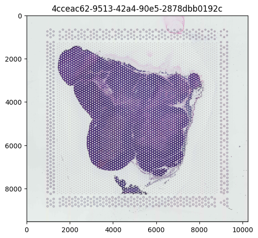
We can use spatialdata-plot to show the H&E stain image. You can refer to the docs page here for more information on the SpatialData plotting API.

[11]:

sdata.pl.render_images().pl.render_shapes().pl.show()

INFO     Rasterizing image for faster rendering.

Clipping input data to the valid range for imshow with RGB data ([0..1] for floats or [0..255] for integers). Got range [0.0..1.008].

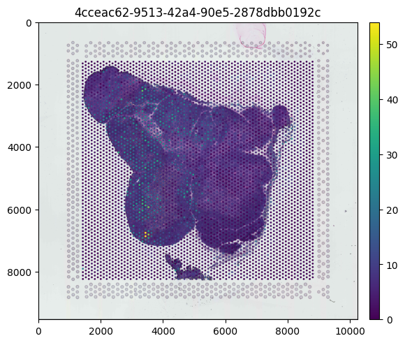
../../_images/notebooks_api_demo_census_spatial_31_2.png

Plotting Continuous Metadata

We can plot expression data over our tissue image from our exported SpatialData object. We can specify various spatial embedding metadata to overlay on the tissue image. Here we plot gene expression of MALAT1, a continuous metadata field.

[12]:

(
    sdata.pl.render_images()
    .pl.render_shapes(color="MALAT1")
    .pl.show()
)

INFO     Rasterizing image for faster rendering.

Clipping input data to the valid range for imshow with RGB data ([0..1] for floats or [0..255] for integers). Got range [0.0..1.008].

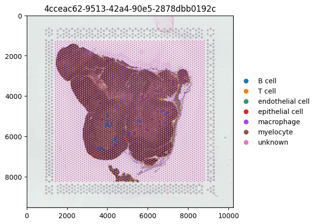
../../_images/notebooks_api_demo_census_spatial_34_2.png

Plotting Categorical Metadata

Below, we will overlay categorical information (cell_type) on our tissue image. When exporting data from the Census, categorical metadata stored in the obs DataFrame is represented as a pandas categorical series.

Since this DataFrame is a subset of the original metadata, its categories still include all possible values from the full Census dataset—even if they are not present in our exported slice of data. This can cause issues when plotting, such as difficulty in automatically assigning a suitable color palette.

To resolve this, we will remove unused categories from the cell_type column before visualization.

[13]:

# Print number of categories before resetting
print("Before:", len(sdata["RNA"].obs["cell_type"].cat.categories))

# Remove unused categories
sdata["RNA"].obs["cell_type"] = sdata["RNA"].obs["cell_type"].cat.remove_unused_categories()

# Print number of categories after resetting
print("After:", len(sdata["RNA"].obs["cell_type"].cat.categories))

Before: 228
After: 7

[14]:

(
    sdata.pl.render_images()
    .pl.render_shapes(color="cell_type")
    .pl.show()
)

INFO     Rasterizing image for faster rendering.

Clipping input data to the valid range for imshow with RGB data ([0..1] for floats or [0..255] for integers). Got range [0.0..1.008].

../../_images/notebooks_api_demo_census_spatial_37_2.png

This should help you get started with accessing, exporting, and visualizing spatial assays retrieved from the CZ CELLxGENE Census. For any feature requests, questions, issues, or help troubleshooting, please reach out to cellxgene@chanzuckerberg.com