CryoET Image Processing Challenges
Overview
Cryo-electron tomography (cryoET) reconstructs 3D volumes, or tomograms, using rotational 2D projections from a sample. In an ideal scenario, each 2D image in a tilt series would represent a true projection of a 3D sample. However, in reality, tomogram reconstructions are based on blurred sample images due to microscope limitations, image acquisition settings, and electron scattering that result in missing, attenuated, or inverted components of true images. This blurring has to be taken into account during image processing to optimize tomogram resolution. Here we discuss major challenges that affect tomogram resolution and analysis, including noisy data, contrast transfer function (CTF), and the tilt angle limitation (“wedge problem”). To provide context for the limitations and their solutions, we’ll first describe how images are processed.
Image Processing: Fourier Space
Researchers transform 2D images into their frequency domain representation using Fourier transforms to enable efficient tomogram reconstruction. Think of an image as a mixture of lots of different patterns – some big and blurry (low resolution), some small and sharp (high resolution). A Fourier transform is a mathematical process that can break down exactly which patterns are present in the image and how strong each one is. These patterns are represented as a combination of different waves, where each wave component describes a particular pattern or level of detail in the image based on their magnitude (strength) and spatial frequency. This information is stored in Fourier space, a representation of the image based on wave patterns. Importantly, researchers can easily convert between Real and Fourier space. Fourier components can be visualized using a power spectrum plot, which depicts the magnitude of each spatial frequency component.
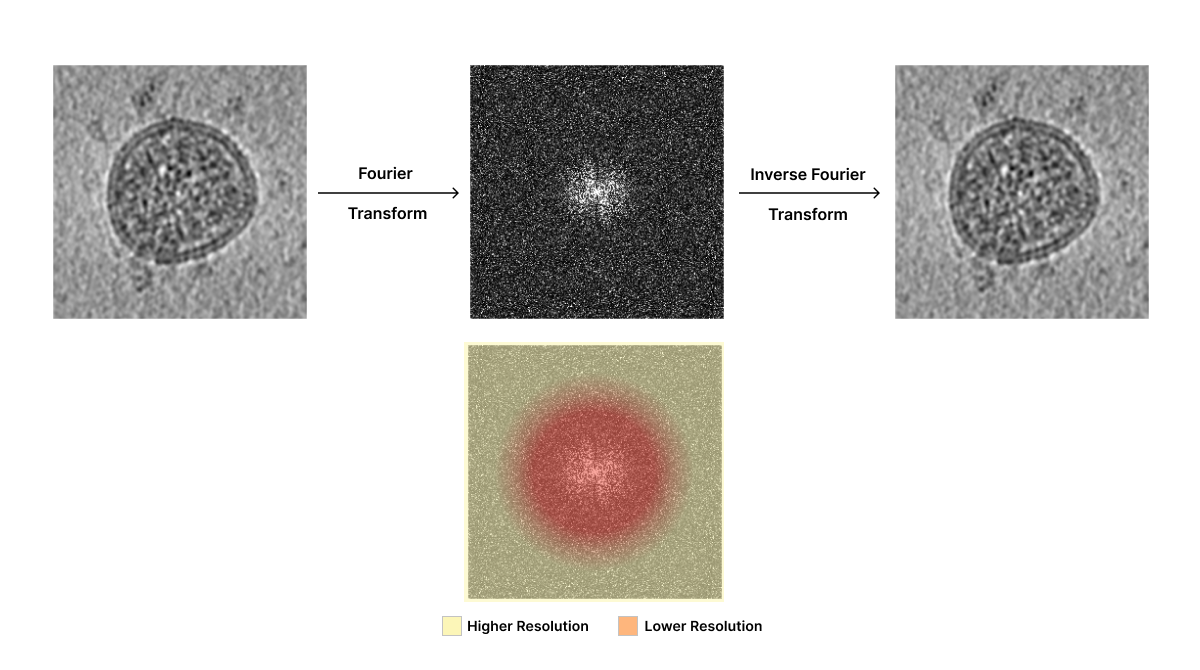
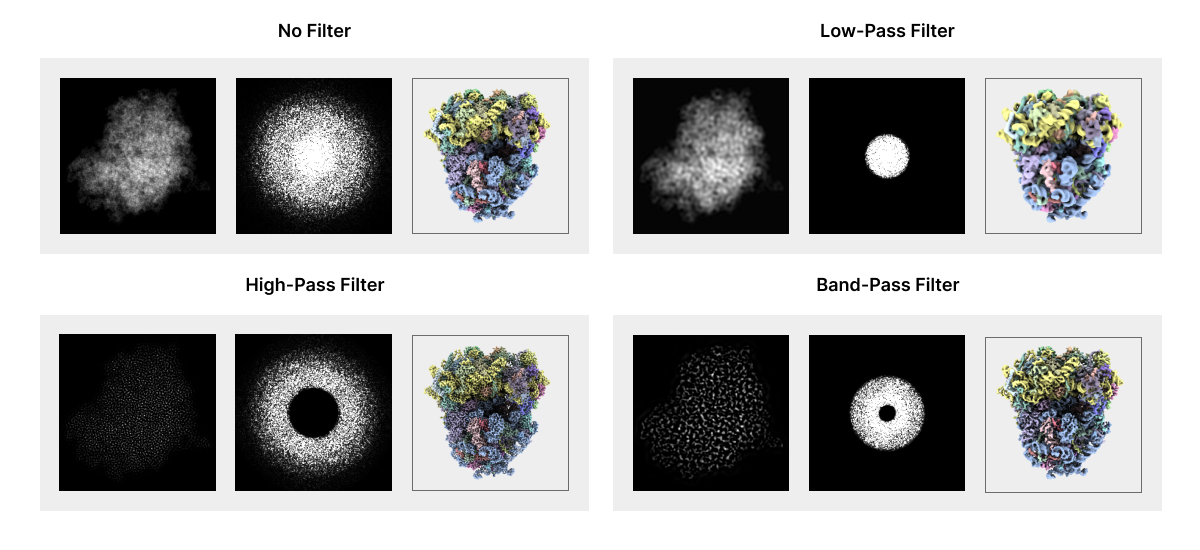
Researchers can take advantage of the Fourier space to manipulate Fourier components that affect the quality of 2D projected images. For example, if you know that most of the “graininess” on an image is made up of tiny white dots of a certain size, you can design a filter that’s really good at removing those specific dots without affecting the actual image too much. Filters can be applied in Fourier space to highlight or remove certain frequency components in the image. Low-pass filters let low-resolution components through and filter out high-resolution image components. Conversely, high-pass filters let high-resolution components through but filter out low-resolution components. Band-filters only retain frequency components within a specified range.
Fourier space enables a number of operations that would be difficult in Real space. Two-dimensional projections obtained through cryo-electron microscopy do not include all the Fourier components that represent true density distributions in the sample due to noise, contrast transfer function, and missing data challenges discussed below. Researchers take advantage of image processing in Fourier space to improve 2D images and, ultimately, tomogram reconstruction despite these limitations.
Noise
CryoET data is inherently noisy. Noise limits the ability to resolve fine tomogram details and can obscure real features in the image, making it difficult to accurately interpret reconstructed structures. Additionally, noise can negatively impact downstream analysis steps, such as segmentation, particle picking and subtomogram averaging.
Noise is introduced during image acquisition and processing. Major sources of noise introduced during image acquisition include:
Sample quality: Imperfections in the vitreous ice embedding of the sample (e.g., contamination) can affect the electron microscope signal and introduce noise.
Sample heterogeneity: Data variability due to complex sample composition can contribute to noise in the reconstruction.
Weak signal: Low electron doses are used to minimize radiation damage to samples. However, these low electron doses result in a weak signal carrying information about the sample. This weak signal is often overwhelmed by noise resulting in a low signal-to-noise ratio (SNR).
Electron scattering: When the electron beam interacts with the sample, electrons are scattered. Elastically scattered electrons retain their energy and provide structural information, whereas inelastically scattered electrons lose energy and introduce random noise. In cryoET, energy filters are used to record elastically scattered electrons but the filters are not perfect and allow some inelastically scattered electrons to pass through.
Radiation damage: Despite low electron doses, radiation damage occurs since total electron beam exposure increases over the course of imaging the sample at various tilt angles. This damage contributes to noise.
Detector noise: The detectors used to capture the electron signal have inherent noise due to electronic noise, variations in pixel sensitivity, and other factors.
Computational methods used to process acquired images and reconstruct the sample 3D volume from 2D projections can also introduce artifacts and noise. This noise can result from limitations in the algorithms or inaccuracies in the tilt series alignment due to differences between individual image projections.
Addressing Noise
Researchers can model noise to remove it from final images. Some of the noise introduced during image acquisition has a statistical distribution that resembles a Gaussian distribution having equal power at all frequencies (“white noise”). This type of noise can be mathematically described to distinguish between real signal (the actual structure of interest) and random fluctuations caused by noise. However, not all noise is white noise. Some noise, known as colored noise, has a complex frequency-dependent power spectrum that is hard to model. Researchers are now implementing machine learning (ML) methods to learn complex noise patterns directly from acquired images and remove them. Below we describe DenoisET, a tool developed by the Chan Zuckerberg Imaging Institute (CZII), to illustrate the application of ML for noise reduction in tomogram reconstructions.
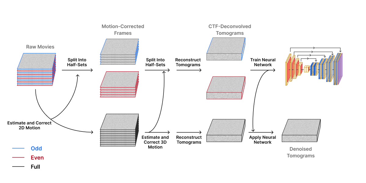
DenoisET is a noise reduction software that leverages an unsupervised convolutional neural network (CNN) known as Noise2Noise. Noise2Noise does not need clean data for training purposes because it “learns to turn bad images into good images by only looking at bad images”. The premise of Noise2Noise is that noisy images have the same underlying clean image but with different noise patterns. The average of noisy images should approximate the denoised image. This is ideal for cryoET image processing where the data is too complex and denoised images are not available for training. DenoisET’s training data includes pairs of reconstructed tomograms derived from pairs of raw movie frames that are used to learn to average out the noise and recover the signal. Once the CNN is trained, it can be applied to denoise tomograms reconstructed from the full dataset.
Contrast Transfer Function
In addition to problems introduced by noise, 2D projections collected through cryoET are not true representations of the original sample. Projected images are affected by electron scattering and microscope optics that result in deviations from true sample representations. These deviations are referred to as aberrations. True image representations would require that all the image Fourier components representing the sample are collected by the electron microscope detector. However, electron scattering and microscope imperfections affect how much contrast each electron that interacts with the sample contributes to the projected image. This means that not all image components are delivered at full contrast during cryoET imaging, thus blurring the image. Aberrations make it difficult to accurately interpret cryoET images given that features in the sample may appear with incorrect contrast or may be completely obscured.
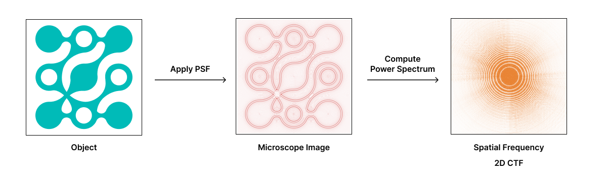
In cryo-electron microscopy, the Point Spread Function (PSF) describes the blurring introduced by the microscope’s optical system, including lens aberrations and defocus, while electron scattering within the sample contributes to contrast loss and limits resolution. The sum of total aberrations generally result in a PSF that consists of oscillating bands of dark and light rings around a single point. The Contrast Transfer Function (CTF) is the Fourier transform of the PSF and describes how different spatial frequencies are transmitted or attenuated by the microscope, affecting image contrast and resolution.
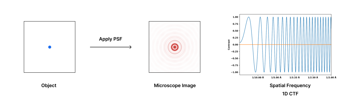
The amplitude of a signal affected by the CTF oscillates and, at certain spatial frequencies, it crosses zero. This means that information at certain spatial frequencies is lost. In some spatial frequencies the CTF is negative leading to contrast information that is reversed at those frequencies. Therefore, the CTF acts as a complex band-filter that distorts the image, making it difficult to accurately interpret the sample’s structure.
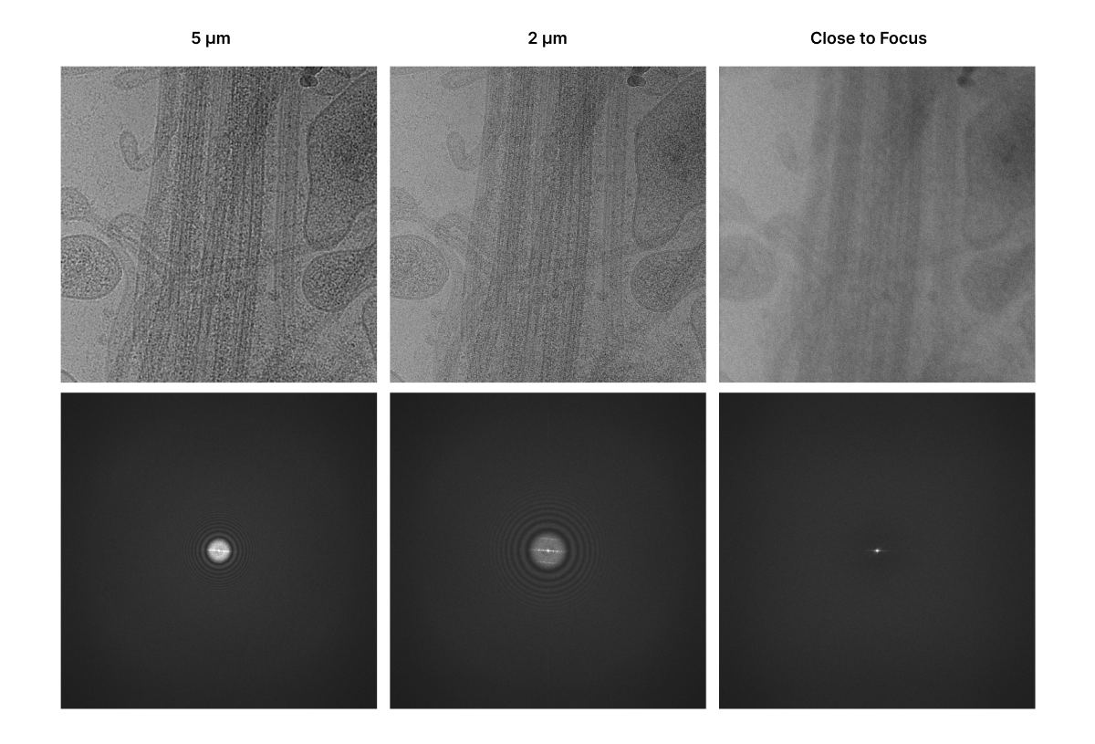
CryoET images are collected out of focus (“defocus”) to improve image contrast (see how cryo-TEM images are formed). Defocus affects the CTF because it shifts which spatial frequency image components contribute to the final image. Taking images with defocus generally increases the magnitude of low spatial frequencies (low resolution features), at the expense of more hard-to-correct oscillations at higher spatial frequencies (high resolution details).
Addressing the CTF
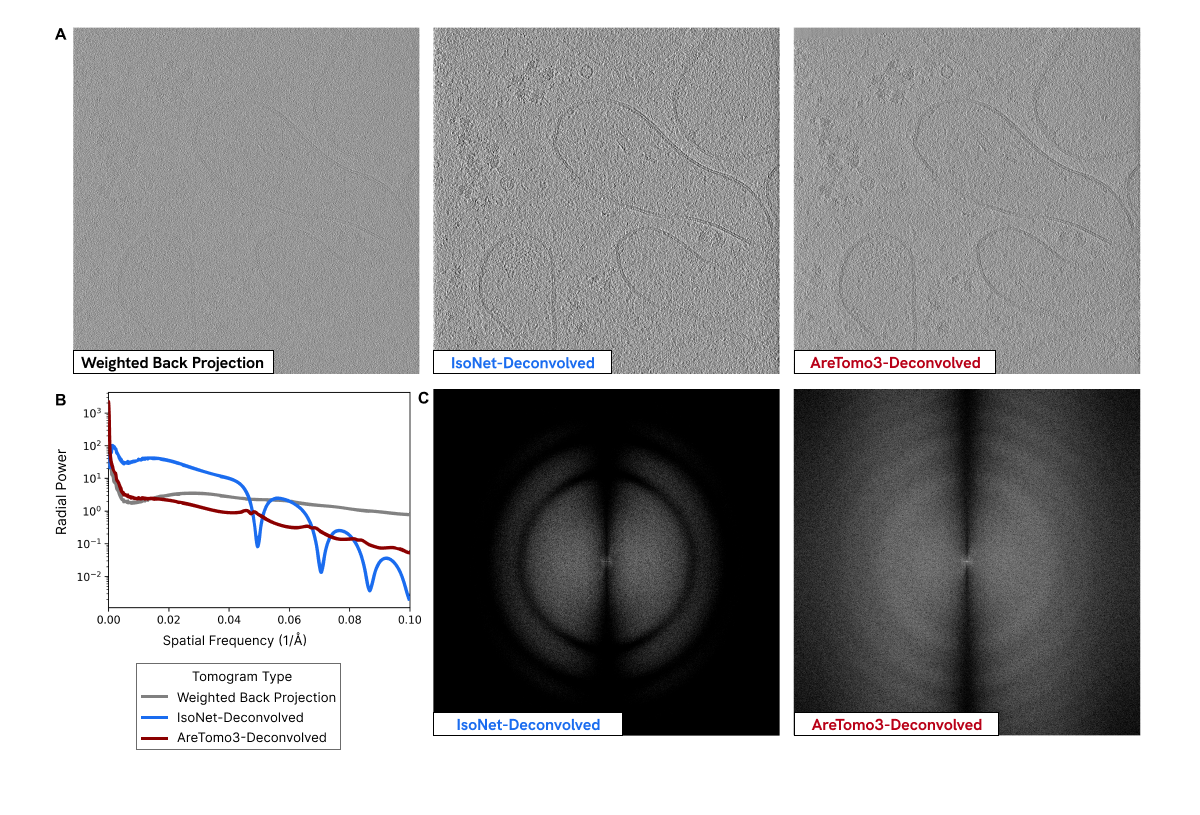
The CTF can be estimated and, therefore, corrected. This is done by primarily determining defocus using the image’s power spectrum, which reveals the CTF’s characteristic oscillations, and other parameters that influence the CTF. Once the CTF is estimated, it can be mathematically reversed through deconvolution. Deconvolution is a computational technique that applies a correction filter to the image’s Fourier transform. This technique compensates for the CTF’s effects and “undoes” the distortions introduced by the microscope.
CTF estimation is a key feature of software packages that preprocess image data for tomogram reconstruction. AreTomo3 enables researchers to preprocess large datasets and reconstruct tomograms in real time. It estimates CTF by integrating GctfFind, a GPU-accelerated implementation of the CTFFIND4 algorithm. This involves an iterative process that implements a theoretical CTF model incorporating parameters that contribute to image distortions (e.g., defocus and spherical aberrations). AreTomo3 systematically varies these parameters to find the best fit between the theoretical CTF model and the experimental power spectrum (i.e., oscillations observed in the power spectrum of collected images). This iterative process helps to find the most accurate CTF parameters that describe the distortions in the image. Once the CTF is modeled with the most accurate parameters, it is corrected using techniques like phase flipping and amplitude correction.
Tilt Angle Limitation (“Missing Wedge” Problem)
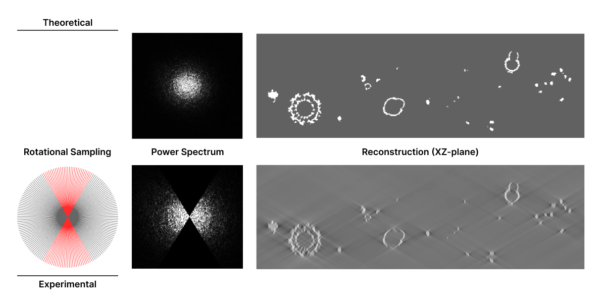
CryoET reconstructs tomograms by combining 2D images of a sample taken at different tilt angles. However, due to hardware limitations, it is not possible to capture a full ±90° range of tilt angles. As the sample tilts, the grid and supporting structures block the electron beam at high angles, and mechanical constraints of the microscope stage further restrict movement, typically limiting tilts to around ±70°. This limitation results in missing data.
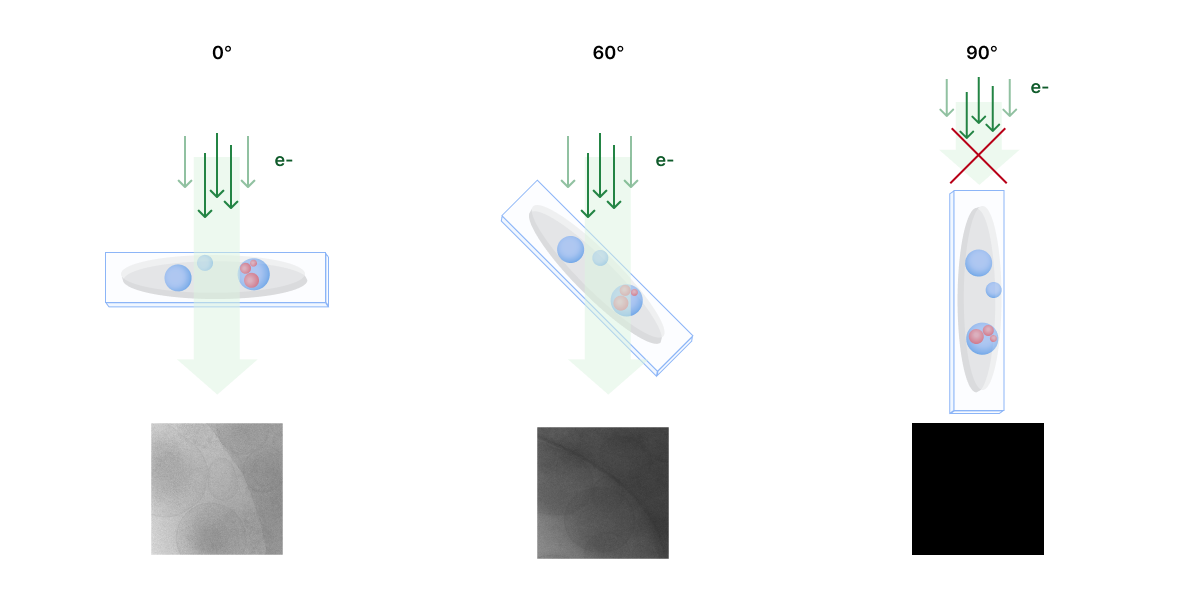
The missing information produces two continuous and opposite wedge-like shapes in the Fourier transform that results in distortion and elongation of the final tomogram reconstruction. Therefore, the tilt angle limitation is commonly referred to as the “missing wedge” problem. Distortions mainly affect structures that are perpendicular to the tilt axis at 0° tilt angle, resulting in omission of top and bottom details in images. This complicates tomogram analysis because it affects the resolution and density accuracy of objects.
Addressing the Missing Wedge Problem
The tilt angle limitation is one of the major challenges in cryoET because insufficient sampling decreases tomogram reconstruction quality and resolution. Due to mechanical constraints, it is hard to address this challenge during image acquisition. However, image processing approaches, such as machine learning, can mitigate reconstruction artifacts produced by the missing wedge problem. Deep neural networks (DNNs) are being trained to learn to predict and restore data in the missing wedge space.
There are different approaches that use supervised and unsupervised DNNs to restore data in the missing wedge space. These DNNs can be trained by comparing different parts of raw tomograms (unsupervised) or using ground-truth data obtained through subtomogram averaging (supervised). Once a DNN is trained, it can be used to fill in the missing information in reconstructed tomograms. This approach has been shown to be effective in reducing the artifacts caused by the missing wedge problem enabling reconstructions that are more accurate and easier to interpret.
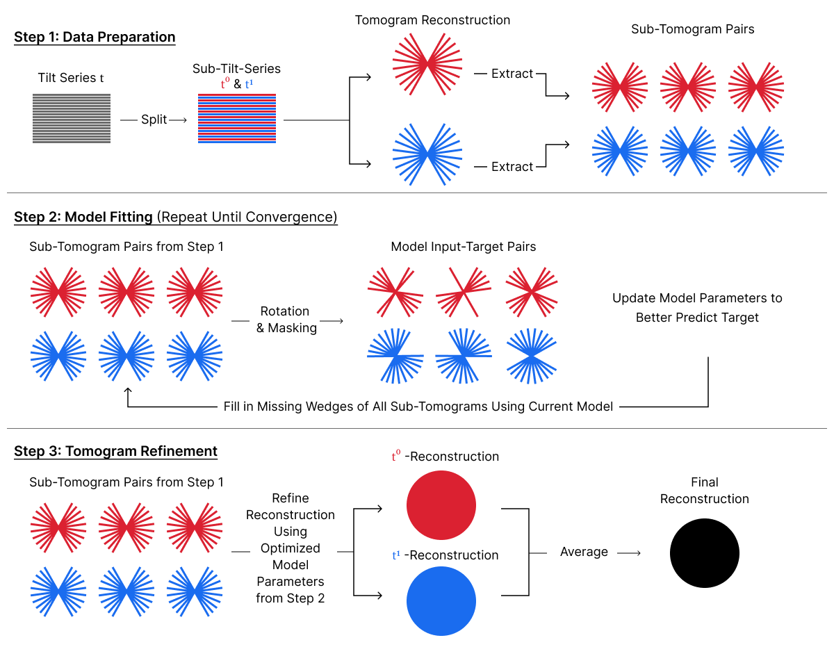
DeepDeWedge is a self-supervised CNN that learns to simultaneously remove noise and fill in the missing wedge from tomograms. It uses motion- and CTF-corrected tilt series as input and splits the data into sub-tomograms to obtain input-target pairs. Similar to Noise2Noise, DeepDeWedge learns to remove noise in reconstructed tomograms from the collected noisy data. Additionally, it increases the diversity of the training data by applying random rotations to sub-tomogram pairs. The sub-tomogram pairs are then used to train the CNN to estimate a noise-free tomogram with a filled-in missing wedge.
Concluding Remarks
In an effort to obtain more accurate representations of imaged samples, researchers are actively improving software and implementing DNNs to enhance tomogram reconstruction. The goal is to restore images closer to what they would have been if noise, CTF, and wedge problem had not introduced any distortions to 3D reconstructions. By addressing these inherent limitations of cryoET data, researchers are significantly enhancing the reliability and interpretability of tomograms to unlock the intricacies of subcellular biological structures.