Training Octopi Models
This guide explains how to train 3D U-Net–based models with Octopi, covering both single-model training and automated model exploration.
Training Modes
Octopi supports two complementary workflows:
-
Single Model Training – Train or fine-tune a specific architecture when you already know what you want.
-
Model Exploration – Automatically search for strong architectures and hyperparameters using Bayesian optimization (recommended for new applications).
Dataset Splitting
For both single-model training and model exploration, Octopi supports training on data drawn from multiple CoPick projects by providing multiple --config files.
You may explicitly control which runs are used for training and validation by specifying --trainRunIDs and --validateRunIDs.
If neither of these options is provided, Octopi automatically:
- Collects all runs that contain both the requested tomograms and the specified segmentation targets
- Splits the data into training and validation sets according to the
--data-splitratio
Single Model Training
For specific use cases or when you have a known good architecture, you can train a single model directly. In this case, the command only allows for training U-Net models. To play around with more unique model configurations, or to try importing new model designs refer to the API or octopi model-explore.
Training New Models
This command initializes a new U-Net model using the specified architecture and training parameters.
octopi train \
    --config config.json \
    --tomo-uri wbp@10.0 \
    --tomo-batch-size 50 --val-interval 10 \
    --target-uri targets:octopi/1
Fine Tuning Models
If we have base weights that we would like to fine-tune for new datasets, we can still use the train command. Instead of specifying the model architecture, we can simply point to the configuration file and weights to load the existing model to fine tune.
octopi train \
    --config config.json \
    --tomo-uri wbp@10.0 \
    --model-config results/model_config.yaml \
    --model-weights results/best_model_weights.pth
octopi train parameters
| Parameter | Description | Example |
|---|---|---|
--config |
One or more CoPick configuration files. Multiple entries may be provided as session_name,path. |
config.json |
--tomo-uri |
Tomogram URI in the form alg@voxel_size. Repeat the flag for multi-resolution training. |
wbp@10.0 |
--target-uri |
Target segmentation in the form name, name:user_id, or name:user_id/session_id. |
targets:octopi/1 |
--trainRunIDs |
Explicit list of run IDs to use for training (overrides automatic splitting). | run1,run2 |
--validateRunIDs |
Explicit list of run IDs to use for validation. | run3,run4 |
--data-split |
Train/validation(/test) split. Single value → train/val, two values → train/val/test. | 0.8 or 0.7,0.1 |
--output |
Directory where model checkpoints, logs, and configs are written. | results |
| Parameter | Description | Default |
|---|---|---|
--num-epochs |
Total number of training epochs. | 1000 |
--val-interval |
Frequency (in epochs) for computing validation metrics. | 10 |
--batch-size |
Number of cropped 3D patches processed per training step. | 16 |
--lr |
Learning rate for the optimizer. | 0.001 |
--best-metric |
Metric used to determine the best checkpoint. Supports fBetaN. |
avg_f1 |
--ncache-tomos |
Number of tomograms cached per epoch (SmartCache window size). | 15 |
--background-ratio |
Foreground/background crop sampling ratio. | 0.0 |
--tversky-alpha |
Alpha parameter for the Tversky loss (foreground weighting). | 0.3 |
Choosing --ncache-tomos
Use this parameter when your dataset has more tomograms than can fit into memory at once — only the cached subset is loaded per epoch, keeping memory usage bounded. Values between 8 and 32 are recommended. Higher values expose the model to more diversity per epoch and improve training throughput, but require more RAM.
| Parameter | Description | Default |
|---|---|---|
--channels |
Feature map sizes at each UNet level. | 32,64,96,96 |
--strides |
Downsampling strides between UNet levels. | 2,2,1 |
--res-units |
Number of residual units per UNet level. | 1 |
--dim-in |
Input patch size in voxels (cube). | 96 |
These options are used to continue training from an existing model.
| Parameter | Description | Example |
|---|---|---|
--model-config |
Model configuration generated by a previous training run. | results/model_config.yaml |
--model-weights |
Pre-trained model weights used for initialization. | results/best_model_weights.pth |
Training Output
During training, you'll see:
- Progress indicators: Real-time loss and accuracy metrics
- Validation results: Periodic evaluation on validation set
- Model checkpoints: Saved to
results/directory by default - Training logs: Detailed logs for monitoring and debugging
Model Exploration
Why Start with Model Exploration?
Rather than manually guessing which learning rates, batch sizes, or architectural choices work best for your specific tomograms, model exploration systematically tests combinations and learns from each trial to make better choices. This automated approach consistently finds better models than manual tuning.
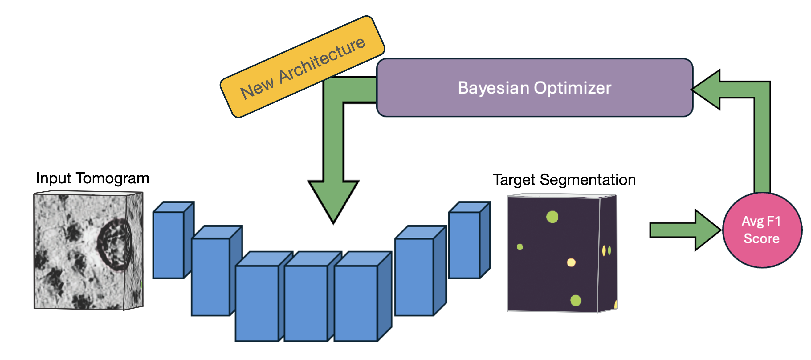 OCTOPI's automated architecture search uses Bayesian optimization to efficiently explore hyperparameters and find optimal configurations for your specific data.
Model exploration is recommended because:
- ✅ No expertise required - Automatically finds the best model for your data
- ✅ Efficient search - Optimal performance tailored to your specific dataset
- ✅ Time savings - Avoids trial-and-error experimentation
Quick Start
octopi model-explore \
    --config config.json \
    --tomo-uri denoised@10.0 \
    --target-uri targets:octopi/1 \
    --data-split 0.7 --model-type Unet \
    --num-trials 100 --best-metric fBeta3 \
    --study-name my-explore-job
This automatically saves results to a timestamped directory and runs 100 optimization trials by default.
octopi model-explore parameters
| Parameter | Description | Default | Notes |
|---|---|---|---|
--config |
One or more CoPick config paths. Multiple entries may be provided as session_name,path. |
– | Use multiple --config entries to combine sessions |
--tomo-uri |
Tomogram URI in the form alg@voxel_size. Repeat the flag for multi-resolution training. |
wbp@10.0 |
Example: --tomo-uri wbp@10.0 --tomo-uri wbp@5.0 |
--target-uri |
Target segmentation: name, name:user_id, or name:user_id/session_id. |
targets:octopi/1 |
From the label preparation step |
--trainRunIDs |
Explicit list of run IDs to use for training (overrides automatic splitting). | – | Example: run1,run2 |
--validateRunIDs |
Explicit list of run IDs to use for validation. | – | Example: run3,run4 |
--data-split |
Train/val(/test) split. Single value → train/val, two values → train/val/test. | 0.8 |
Example: 0.7,0.1 → 70/10/20 |
--output |
Name/path of the output directory. | explore_results |
Results are written here per study |
--study-name |
Name of the Optuna/MLflow experiment. | model-search |
Useful for organizing runs |
| Parameter | Description | Default | Notes |
|---|---|---|---|
--model-type |
Model family used for exploration. | Unet |
Options: unet, attentionunet, mednext, segresnet |
--num-epochs |
Number of epochs per trial. | 1000 |
Consider fewer epochs for quick sweeps |
--val-interval |
Validation frequency (every N epochs). | 10 |
Smaller = more frequent metrics |
--ncache-tomos |
Number of tomograms cached per epoch (SmartCache window size). | 15 |
Higher values improve throughput but require more memory |
--best-metric |
Metric used to select the best checkpoint (supports fBetaN). |
avg_f1 |
Example: fBeta3 emphasizes recall |
--background-ratio |
Foreground/background crop sampling ratio. | 0.0 |
1.0 → 50/50; <1.0 biases toward foreground |
Choosing --ncache-tomos
Use this parameter when your dataset has more tomograms than can fit into memory at once — only the cached subset is loaded per epoch, keeping memory usage bounded. Values between 8 and 32 are recommended. Higher values expose the model to more diversity per epoch and improve training throughput, but require more RAM.
| Parameter | Description | Default | Notes |
|---|---|---|---|
--num-trials |
Number of Optuna trials (models) to evaluate. | 100 |
Use 50-200 for sufficient exploration of the parameter landscape. |
--random-seed |
Random seed for reproducibility. | 42 |
Fix this when comparing changes |
| Parameter | Description | Default | Notes |
|---|---|---|---|
--submitit |
Submit trials as independent SLURM jobs using submitit instead of running locally. | False |
Enables HPC / multi-node execution |
--njobs |
Maximum number of concurrent SLURM jobs (trials) to run at once. | 5 |
Each job runs exactly one Optuna trial |
--compute-constraint |
CPU and memory request per SLURM job in the form cpus,mem_gb. |
4,16 |
Example: 8,32 requests 8 CPUs and 32 GB RAM |
--timeout |
Walltime limit (hours) per SLURM job. | 4 |
Jobs exceeding this limit are terminated by the scheduler |
What changes when --submitit is enabled?
By default, octopi model-explore runs locally, launching one worker per available GPU and executing multiple trials within a single process.
When --submitit is enabled, Octopi switches to a job-based execution model designed for SLURM-HPC clusters:
- Each Optuna trial is executed as a separate SLURM job
- Jobs may run on different nodes and start at different times
- Resource limits (CPUs, memory, walltime) are enforced per trial
- Failed jobs affect only the corresponding trial, not the entire study
This mode provides better scalability and fault isolation for large model exploration runs, especially on shared HPC systems.
Because multiple jobs may write to the same Optuna and MLflow tracking databases, Octopi uses best-effort retries for database operations to safely handle temporary contention.
What Gets Optimized?
Model exploration uses fixed architectures with two available options:
- Unet - Standard 3D U-Net (default, recommended for most cases)
- AttentionUnet - U-Net with attention mechanisms (for complex data)
For each architecture, it optimizes:
- Hyperparameters - Learning rate, batch size, loss function parameters
- Architecture details - Channel sizes, stride configurations, residual units
- Training strategies - Regularization and data augmentation
Parallelism and GPU Utilization
When running octopi model-explore, Octopi automatically detects the available GPU resources and spawns one worker per GPU. Each worker independently trains a candidate model, allowing multiple Optuna trials to run concurrently.
This means:
- On a machine with N GPUs, up to N models are trained in parallel
- Trial scheduling is handled automatically by Optuna
- GPU utilization scales naturally from a single workstation to multi-GPU HPC nodes
On shared HPC systems, the number of concurrent trials is therefore determined by the number of GPUs allocated to your job (e.g., via Slurm or another scheduler).
Note
If fewer GPUs are available than the total number of trials (--num-trials), remaining trials are queued and executed as workers become free.
Monitoring Your Training
Track the progress of model exploration runs in real time, inspect trial performance, and understand which hyperparameters and architectural choices drive model quality.
Octopi integrates with Optuna to provide a high-level view of the architecture and hyperparameter search process. This dashboard is best suited for understanding which trials perform best, which parameters matter most, and how the optimization converges over time.
Setup Options:
-
Web Dashboard – Launch the Optuna dashboard directly from the command line:
BashReplaceoptuna-dashboard sqlite:///{path-to}/trials.dbpath/to/trials.dbwith the path to the Optuna study database located in the model exploration output directory. -
VS Code Extension - Install Optuna extension for integrated monitoring, right click on
trials.dbin the file navigator to launch the dashboard.
What you'll see:
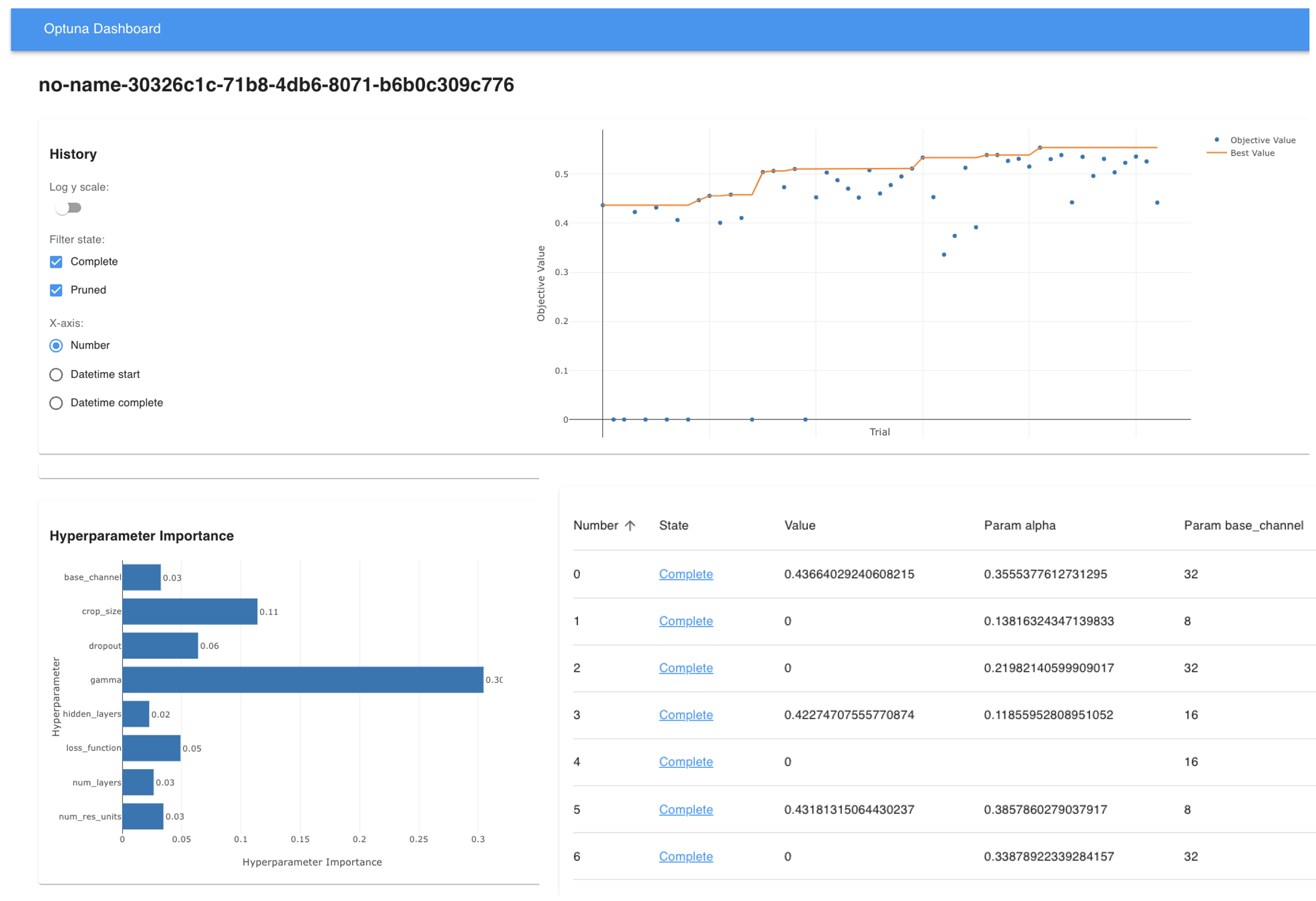
- Trial progress and current best performance
- Parameter importance (which settings matter most)
- Optimization history and convergence trends
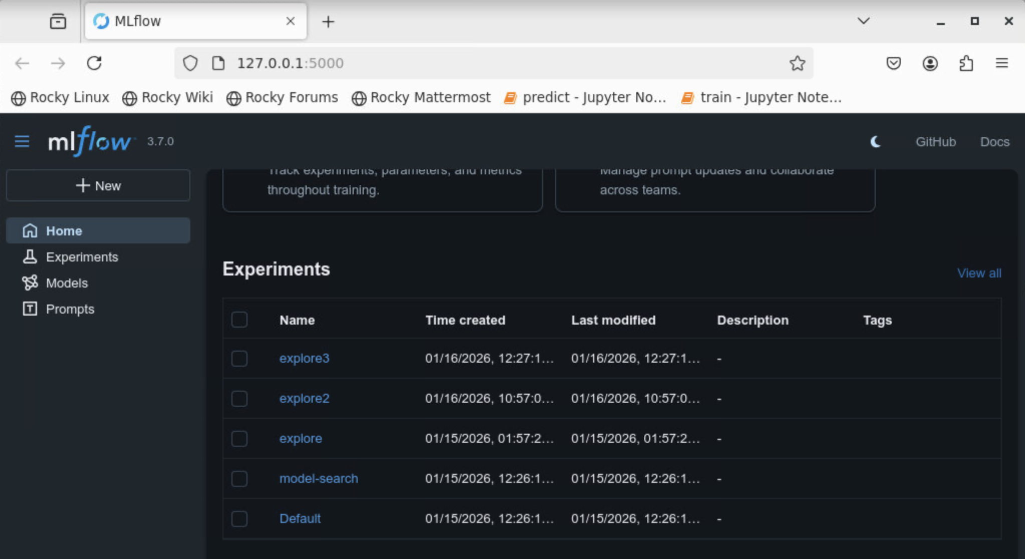
MLflow complements Optuna by providing detailed, per-trial training information, including loss curves, validation metrics, model checkpoints, and configuration artifacts.
If you are running octopi model-explore on your local machine, start the MLflow UI in the same environment:
mlflow ui
If the mlflow command is not directly available, use the alternative:
python -m mlflow ui
This will print output similar to:
INFO: Uvicorn running on http://127.0.0.1:5000
Copy the URL and paste it into your browser to open the MLflow dashboard.
When octopi is executed on a remote HPC system, the MLflow UI runs on a machine that is not directly accessible from your local browser. To view it locally, you must forward the MLflow port using an SSH tunnel.
On your local machine, open a terminal and run:
ssh -L 5000:localhost:5000 username@login-node-hostname
This creates an SSH tunnel to the HPC login node and forwards port 5000 to your local machine.
Once logged in, navigate to the directory where the model exploration results are being written. You should see files such as:
mlflow.db
mlruns/
These files define the MLflow experiment state. From this directory, start the MLflow UI:
python -m mlflow ui --host 0.0.0.0 --port 5000
Finally, on your local machine, open the following address in your browser:
http://127.0.0.1:5000
When the dashboard is opened, you should now see the MLflow experiment associated with your study-name specified when running the job.
Model Exploration Output
- Optuna study database
- MLflow experiment logs
- Best-performing model checkpoints
- Per-trial metrics and configurations
Class Weighting
When training on datasets with multiple particle types, some classes may be more important to detect than others — or should be excluded from scoring entirely. Octopi supports per-class weights read directly from the CoPick configuration file, so no additional training flags are needed.
Weights are applied in two places:
- Training — the validation F-beta score is computed as a weighted average across classes, so checkpoint selection favors performance on higher-weight classes.
- Evaluation —
octopi evaluateuses the same weights when reporting aggregate metrics.
How to set weights in your CoPick config
Add a metadata field to any pickable_object entry in your config.json with a weight key:
{
    "name": "ribosome",
    "is_particle": true,
    "label": 4,
    "radius": 150,
    "metadata": {
        "weight": 2
    }
}
If metadata or weight is absent for a class, it defaults to 1. Set weight to 0 to exclude a class from scoring entirely.
The following config weights beta-galactosidase and thyroglobulin twice as heavily as apoferritin and ribosome, and excludes beta-amylase from scoring:
{
    "pickable_objects": [
        {
            "name": "apoferritin",
            "is_particle": true,
            "label": 1,
            "radius": 60,
            "metadata": { "weight": 1 }
        },
        {
            "name": "beta-amylase",
            "is_particle": true,
            "label": 2,
            "radius": 80,
            "metadata": { "weight": 0 }
        },
        {
            "name": "beta-galactosidase",
            "is_particle": true,
            "label": 3,
            "radius": 90,
            "metadata": { "weight": 2 }
        },
        {
            "name": "ribosome",
            "is_particle": true,
            "label": 4,
            "radius": 150,
            "metadata": { "weight": 1 }
        },
        {
            "name": "thyroglobulin",
            "is_particle": true,
            "label": 5,
            "radius": 130,
            "metadata": { "weight": 2 }
        }
    ]
}
Tip
Weights only affect the validation metric used for checkpoint selection and the aggregate evaluation score — the loss function and per-class metrics are unaffected.
Compute & Performance
Three levers cover the most common issues:
Out-of-memory (OOM)
The quickest fix for a RAM OOM is to increase total memory. On SLURM, bump --mem-per-cpu — raising from 8G to 12G on a 16-CPU allocation adds 64 GB with no other changes needed. If that's not enough, lower --ncache-tomos to reduce how much data is held in RAM at once (see below).
For GPU OOMs, lower --batch-size first (the biggest VRAM lever), then --dim-in if still needed (96 → 64 cuts activation memory ~3.4×).
SLURM: more CPUs, modest memory per CPU
DataLoader workers are the main training throughput bottleneck — more CPUs keep the GPU fed. Each worker only needs a moderate amount of RAM, so request more CPUs rather than a large per-CPU allocation:
#SBATCH --cpus-per-task=16
#SBATCH --mem-per-cpu=8G      # 128 GB total — sufficient for most datasets
#SBATCH --gpus=1
If you're caching many tomograms or hitting RAM OOMs, bump --mem-per-cpu to 12G (192 GB total) before reducing CPU count. Octopi automatically matches the number of DataLoader workers to --cpus-per-task at runtime.
Tuning epoch time with --ncache-tomos
--ncache-tomos controls how many tomograms are held in RAM at once (the SmartCache window). On large datasets — where loading every tomogram up front would be slow or exhaust RAM — this is the primary lever for controlling epoch duration: a smaller cache means fewer tomograms are swapped in and out per epoch, so each epoch completes faster.
The tradeoff is data diversity: a smaller window means the model sees fewer unique tomograms per epoch and may need more epochs to converge. Values between 8 and 32 work well for most datasets — start at the default (15) and decrease if epochs are taking too long or if you're running low on RAM.
- Validation adds a sticky baseline. First-time validation expands the CUDA caching allocator, imports code paths for the first time, creates a long-lived matplotlib figure, and builds class-index caches. None of this is released.
Together, these mean main-process RAM grows over the first few epochs and then plateaus. If that plateau + per-epoch worker drift ≈ cgroup limit, you OOM. The fix is more RAM, less drift (fewer workers, smaller cache), or less baseline (smaller val_batch_size).
Next Steps
After training is complete:
Run inference - Apply your best model to new tomograms and get particle locations from predictions.