Normalizing full-length gene sequencing data

This tutorial shows you how to fetch full-length gene sequencing data from the Census and normalize it to account for gene length.

Contents

1. Opening the census

2. Fetching example full-length sequencing data (Smart-Seq2)

3. Normalizing expression to account for gene length

4. Validation through clustering exploration

⚠️ Note that the Census RNA data includes duplicate cells present across multiple datasets. Duplicate cells can be filtered in or out using the cell metadata variable is_primary_data which is described in the Census schema. For this notebook we will focus on individual datasets, therefore we can ignore this variable.

Opening the census

First we open the Census, if you are not familiar with the basics of the Census API you should take a look at notebook Learning about the CZ CELLxGENE Census

import cellxgene_census
import scanpy as sc
from scipy.sparse import csr_matrix

census = cellxgene_census.open_soma()

The "stable" release is currently 2023-07-25. Specify 'census_version="2023-07-25"' in future calls to open_soma() to ensure data consistency.

You can learn more about the all of the cellxgene_census methods by accessing their corresponding documention via help(). For example help(cellxgene_census.open_soma).

Fetching full-length example sequencing data (Smart-Seq)

Let’s get some example data, in this case we’ll fetch all cells from a relatively small dataset derived from the Smart-Seq2 technology which performs full-length gene sequencing:

• Collection: Tabula Muris Senis

• Dataset: Liver - A single-cell transcriptomic atlas characterizes ageing tissues in the mouse - Smart-seq2

Let’s first find this dataset’s id by using the dataset table of the Census

liver_dataset = (
    census["census_info"]["datasets"]
    .read(
        value_filter="dataset_title == 'Liver - A single-cell transcriptomic atlas characterizes ageing tissues in the mouse - Smart-seq2'"
    )
    .concat()
    .to_pandas()
)
liver_dataset

	soma_joinid	collection_id	collection_name	collection_doi	dataset_id	dataset_title	dataset_h5ad_path	dataset_total_cell_count
0	525	0b9d8a04-bb9d-44da-aa27-705bb65b54eb	Tabula Muris Senis	10.1038/s41586-020-2496-1	4546e757-34d0-4d17-be06-538318925fcd	Liver - A single-cell transcriptomic atlas cha...	4546e757-34d0-4d17-be06-538318925fcd.h5ad	2859

Now we can use this id to fetch the data.

liver_dataset_id = "4546e757-34d0-4d17-be06-538318925fcd"
liver_adata = cellxgene_census.get_anndata(
    census,
    organism="Mus musculus",
    obs_value_filter=f"dataset_id=='{liver_dataset_id}'",
)

Let’s make sure this data only contains Smart-Seq2 cells

liver_adata.obs["assay"].value_counts()

assay
Smart-seq2    2859
Name: count, dtype: int64

Great! As you can see this a small dataset only containing 2,859 cells. Now let’s proceed to normalize by gene lengths.

For good practice let’s add the number of genes expressed by cell, and the total counts per cell.

Don’t forget to close the census

census.close()

Normalizing expression to account for gene length

By default cellxgene_census.get_anndata() fetches all genes in the Census. So let’s first identify the genes that were measured in this dataset and subset the AnnData to only include those.

To this goal we can use the “Dataset Presence Matrix” in census["census_data"]["mus_musculus"].ms["RNA"]["feature_dataset_presence_matrix"]. This is a boolean matrix N x M where N is the number of datasets and M is the number of genes in the Census, True indicates that a gene was measured in a dataset.

liver_adata.n_vars

52392

Let’s get the genes measured in this dataset.

liver_dataset_id = liver_dataset["soma_joinid"][0]

presence_matrix = cellxgene_census.get_presence_matrix(census, "Mus musculus", "RNA")
presence_matrix = presence_matrix[liver_dataset_id, :]
gene_presence = presence_matrix.nonzero()[1]

liver_adata = liver_adata[:, gene_presence].copy()

liver_adata.n_vars

17992

We can see that out of the all genes in the Census 17,992 were measured in this dataset.

Now let’s normalize these genes by gene length. We can easily do this because the Census has gene lengths included in the gene metadata under feature_length.

liver_adata.X[:5, :5].toarray()

array([[0.000e+00, 0.000e+00, 0.000e+00, 0.000e+00, 0.000e+00],
       [0.000e+00, 0.000e+00, 5.590e+02, 0.000e+00, 0.000e+00],
       [0.000e+00, 0.000e+00, 1.969e+03, 0.000e+00, 8.280e+02],
       [0.000e+00, 0.000e+00, 0.000e+00, 0.000e+00, 1.000e+00],
       [0.000e+00, 2.250e+03, 0.000e+00, 0.000e+00, 5.400e+01]],
      dtype=float32)

gene_lengths = liver_adata.var[["feature_length"]].to_numpy()
liver_adata.X = csr_matrix((liver_adata.X.T / gene_lengths).T)

liver_adata.X[:5, :5].toarray()

array([[0.00000000e+00, 0.00000000e+00, 0.00000000e+00, 0.00000000e+00,
        0.00000000e+00],
       [0.00000000e+00, 0.00000000e+00, 6.58654413e-02, 0.00000000e+00,
        0.00000000e+00],
       [0.00000000e+00, 0.00000000e+00, 2.32001885e-01, 0.00000000e+00,
        2.74444813e-01],
       [0.00000000e+00, 0.00000000e+00, 0.00000000e+00, 0.00000000e+00,
        3.31455088e-04],
       [0.00000000e+00, 4.71500419e-01, 0.00000000e+00, 0.00000000e+00,
        1.78985747e-02]])

All done! You can see that we now have real numbers instead of integers.

Validation through clustering exploration

Let’s perform some basic clustering analysis to see if cell types cluster as expected using the normalized counts.

First we do some basic filtering of cells and genes.

sc.pp.filter_cells(liver_adata, min_genes=500)
sc.pp.filter_genes(liver_adata, min_cells=5)

Then we normalize to account for sequencing depth and transform data to log scale.

sc.pp.normalize_total(liver_adata, target_sum=1e4)
sc.pp.log1p(liver_adata)

Then we subset to highly variable genes.

sc.pp.highly_variable_genes(liver_adata, n_top_genes=1000)
liver_adata = liver_adata[:, liver_adata.var.highly_variable].copy()

And finally we scale values across the gene axis.

sc.pp.scale(liver_adata, max_value=10)

Now we can proceed to do clustering analysis

sc.tl.pca(liver_adata)
sc.pp.neighbors(liver_adata)
sc.tl.umap(liver_adata)
sc.pl.umap(liver_adata, color="cell_type")

/home/ssm-user/cellxgene-census/venv/lib/python3.10/site-packages/tqdm/auto.py:21: TqdmWarning: IProgress not found. Please update jupyter and ipywidgets. See https://ipywidgets.readthedocs.io/en/stable/user_install.html
  from .autonotebook import tqdm as notebook_tqdm
/home/ssm-user/cellxgene-census/venv/lib/python3.10/site-packages/scanpy/plotting/_tools/scatterplots.py:392: UserWarning: No data for colormapping provided via 'c'. Parameters 'cmap' will be ignored
  cax = scatter(

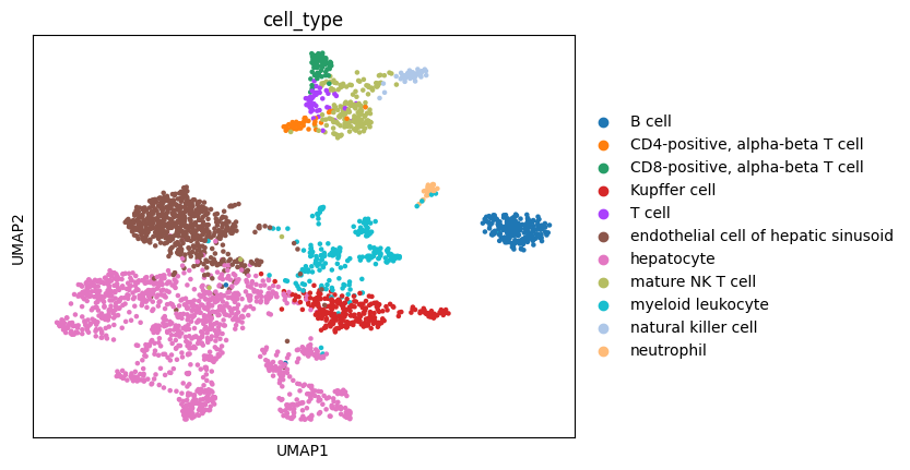
With a few exceptions we can see that all cells from the same cell type cluster near each other which serves as a sanity check for the gene-length normalization that we applied.